Regression 7. Understanding Non-linear Regression with Polynomial Curve fitting
Polynomial Curve Fitting
Polynomial
curve fitting is a statistical technique used to model a relationship between a
dependent variable and one or more independent variables using a polynomial
equation. This approach is particularly useful when the relationship between
the variables is non-linear and cannot be adequately described by a simple
linear model.
Example
Create
a dataset with one independent variable x and a dependent variable denoted by
sin(2πx).
|
x |
0 |
0.1 |
0.2 |
0.3 |
0.4 |
0.5 |
0.6 |
0.7 |
0.8 |
0.9 |
1 |
|
sin(2πx) |
0 |
0.5878 |
0.9511 |
0.9511 |
0.5878 |
0 |
-0.5878 |
-0.9511 |
-0.9511 |
-0.5878 |
0 |
|
x |
|
1.1 |
1.2 |
1.3 |
1.4 |
1.5 |
1.6 |
1.7 |
1.8 |
1.9 |
2 |
|
sin(2πx) |
|
0.5878 |
0.9511 |
0.9511 |
0.5878 |
0 |
-0.5878 |
-0.9511 |
-0.9511 |
-0.5878 |
0 |
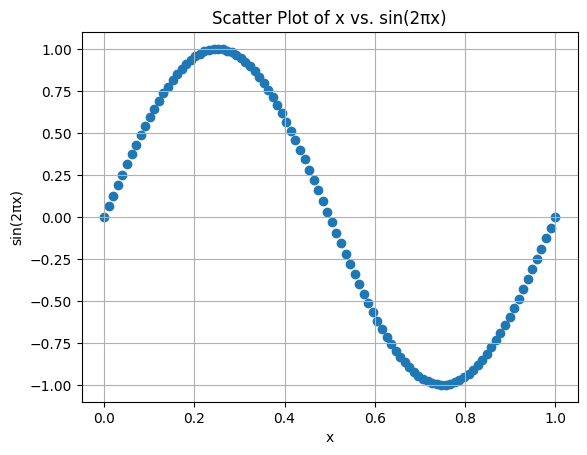
Relationship between Variables
The relationship between the variables is not linear as
shown in the following graph.
Task:
The task is to learn the equation that shows the relationship between the input(x) and output (2πx).
Polynomial Equation
So we can use a polynomial equation to represent the relationship.

Polynomial Approximations of sin(2πx) of Varying Degrees
p(x) = -4.1585x^3 + 4.1585x
p(x) = -4.9348x^5 + 9.8696x^3 - 4.9348x
p(x) = -28.2743x^9 + 126.0972x^7 - 252.1944x^5 + 201.7552x^3 - 67.2517x
Note that the co-efficients increase drastically as the degree increases.
Degree and Co-efficient of Polynomial
The co-efficient is learnt by the machine learning model. But assumptions have to be made on the degree of the polynomial.
Adding Noise to Dataset
If the exact equation is learnt while creating the machine learning model, the prediction on unseen data is low. So we can add noise to the data so that the machine learns the pattern ignoring the noise.

When degree = 0,

A polynomial of degree 0 is essentially a constant value (a horizontal line) that best fits the data in the least squares sense. This is equivalent to finding the mean of the y values in the dataset.
When degree = 1,
any straight line can be learnt by the model. It does not understand even the training dataset and so it results in underfitting.

When degree = 3,


When degree = 9,
it learns the points in dataset and not the underlying pattern in the dataset. This results in overfitting. It can predict any example in the training set correctly. But is cannot predict well on unseen data.
Fitting a polynomial of degree 9 to your data is an advanced task, as it involves finding a high-degree polynomial that can closely follow the patterns (and potentially the noise) in your data.

Degree 25

Polynomial Curve Fitting with an ANN using pytorch can be with example in the following YouTube video.
Comments
Post a Comment