Machine Learning - Simplified

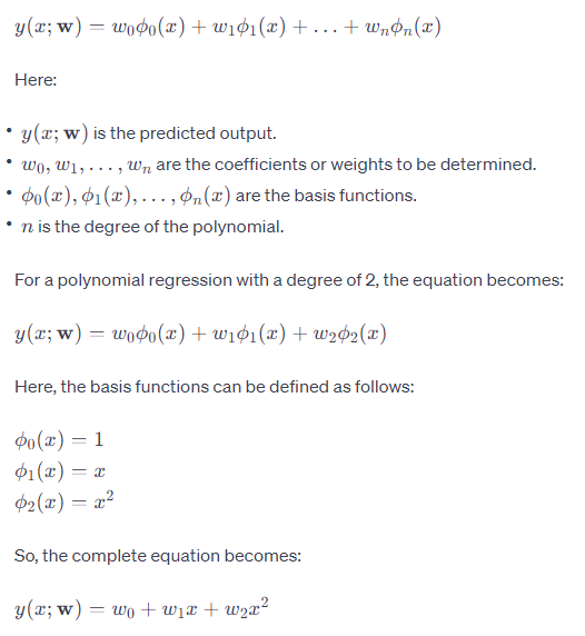
We create models making approximations on the equation that would fit a training set. Some common approximations we make are linear(y=W.X), polynomial(given in notes). How do we validate our model approximation? A good model should neither underfit(simple models) nor overfit(complex models).  Bias Bias shows if a model has a tendency to underfit. To measure bias we create models on different training datasets using k-fold cross validation and measure how much the predicted values of the models created differ from the true value. If they underfit, the models created will be similar and the mean of the predicted values will vary a lot from the true value. That is, they have high bias. A model that fits well will have low bias. Variance On the other hand, variance measures if a model has the tendency to overfit. It checks how much the models created in k-fold cross-validation differ from one another. If they overfit, the variance between the predicted models will be high. This normally ha

 Numeric Example A hypothetical dataset about how online gaming habits affects marks involving children in the age group of 10-15 is tabulated. The first feature is the number of hours in a day spent in gaming. The second feature gives the average marks of the students who spend so many hours in gaming. Problem Statement Find the regression coefficients w0 and w1 in the linear regression model using Least Squares Approach: y = w0+ w1*x

Pseudo-Inverse Matrix Approach: The pseudo-inverse matrix approach is essentially the OLS approach. It provides a solution to the linear regression problem by minimizing the sum of squared residuals between the observed and predicted values. This approach is a direct algebraic method that does not make any probabilistic assumptions about the residuals; it simply finds the best fit in the least squares sense.   For simple linear regression, the MLE estimates of the coefficients will actually be the same as the Ordinary Least Squares (OLS) estimates, which are also the same as what you get from the pseudo-inverse matrix method, under the assumption of i.i.d. normal errors. In this blog we show how to prove that  Maximization of likelihood function under conditional Gaussian noise for a linear model is similar to the minimization of the sum of the squares error function.  The complete derivation along with formulae used are provided. Ensure that you go through the previous blogs to get a

  MLE Approach: When performing linear regression using MLE under the assumption that the residuals (errors) are independently and identically distributed (i.i.d.) with a normal distribution, we estimate the regression coefficients that maximize the likelihood of observing the given data. In this blog we see how to perform regression on a dataset that applies MLE for model fitting. The mathematical assumptions and derivations are given in detail.   The MLE approach gives you point estimates for the coefficients (mean of the likelihood distribution), and you can also compute the variance-covariance matrix of these estimates, which gives you the variances (and covariances) of the estimates. These variances are a measure of the uncertainty or the spread of the likelihood distribution of the parameter estimates. For simple linear regression, the MLE estimates of the coefficients will actually be the same as the Ordinary Least Squares (OLS) estimates, which are also the same as what you get

Introduction For polynomial curve fitting, you can use basis functions to model the relationship between the input features and the output variable .  General Form The general form of a polynomial regression equation with basis functions is: Each term in the equation is the product of a weight and a basis function evaluated at the input x . The basis functions capture the polynomial terms of different degrees, allowing the model to fit more complex curves to the data. Quadratic and cubic Polynomials for Scalar x Polynomial for Vectors The basis functions are : 

 Polynomial Curve Fitting Polynomial curve fitting is a statistical technique used to model a relationship between a dependent variable and one or more independent variables using a polynomial equation . This approach is particularly useful when the relationship between the variables is non-linear and cannot be adequately described by a simple linear model. Example Create a dataset with one independent variable x and a dependent variable denoted by sin(2πx). x 0 0.1 0.2 0.3 0.4 0.5 0.6 0.7 0.8 0.9 1 sin(2 πx ) 0 0.5878 0.9511 0.9511 0.5878 0 -0.5878 -0.9511 -0.9511 -0.5878 0   x   1.1 1.2 1.3 1.4 1.5 1.6 1.7 1.8 1.9 2 sin(2 πx )